Step by step noise analysis for planners and consultants
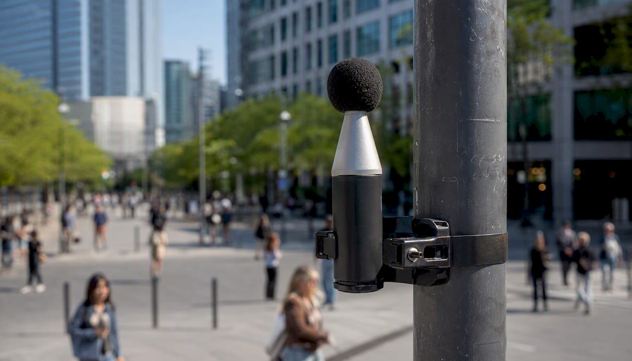
Step by step noise analysis follows a fixed sequence: define scope and indicators, gather and audit input datasets, choose a calculation method, run and calibrate the model, produce decision-ready outputs, test mitigation scenarios, then quality-check and report. The deliverable planners need is a CNOSSOS‑EU-compliant noise map (where EU strategic mapping applies), calibrated against measured data, with receiver exposure tables and scenario comparison graphics ready for stakeholders. Open tools such as NoiseModelling handle the calculation engine; a digital twin platform like 3D Cityplanner handles the 3D visualisation and scenario testing that turns numbers into decisions.
- Define scope, indicators and receivers
- Collect and audit input datasets
- Select method and software
- Model, calibrate, report uncertainty
- Produce maps and exposure statistics
- Test mitigation scenarios in 3D
- Quality-check and finalise reporting
Key Takeaways
Step by step noise analysis works because each stage, from scope definition through calibration to scenario testing, feeds directly into the next, and skipping one weakens every result that follows.
| Point | Details |
|---|---|
| Fix scope before modelling | Decide strategic map versus site assessment, indicators and receivers before touching any dataset. |
| Audit dataset age | Keep road, rail, aircraft and building data within roughly three years, and document sources. |
| Calibrate against measurement | Use 24‑hour monitoring where practical and apply documented correction factors to the model. |
| Report vertical and delta results | Deliver façade exposure plots and scenario delta maps, not just ground-level contours. |
| Test mitigation in 3D | Platforms like 3D Cityplanner let planners compare massing, barrier and planting scenarios visually before construction. |
Table of Contents
- When to run a strategic noise map versus a site-level impact assessment
- Step 1: Define objectives, indicators and scope
- Step 2: Gather and prepare your input datasets
- Step 3: Choose the right calculation method and tools
- Step 4: Run the model, calibrate and report uncertainty
- Step 5: Produce maps, exposure tables and decision-ready graphics
- Step 6: Test mitigation scenarios and compare results in 3D
- Quality assurance, reporting and common pitfalls
- Pre-delivery checklist for reports and stakeholder meetings
- Why acoustics belongs in masterplanning, not compliance
- How a 3D digital twin speeds up your workflow
- Sources
- FAQ
When to run a strategic noise map versus a site-level impact assessment
Strategic noise mapping covers whole urban areas, uses annual-average indicators, and feeds five-year reporting cycles under the Environmental Noise Directive. Site-level impact assessments answer a narrower question: what will residents on the third floor of a proposed block actually hear, and does that exceed local thresholds for a planning application.
- Strategic maps: use Lden and Lnight, area-wide grids, updated on END reporting cycles.
- Site assessments: use Leq, LFmax and façade-by-façade profiles, tied to a specific project timeline.
- Regulatory use: strategic maps support action plans; site assessments support planning consent and design mitigation.
Mixing the two up is the most common early mistake. A developer asking whether a proposed tower will breach façade noise limits doesn’t need an area-wide Lden grid, they need receiver-height accuracy at the actual building line.
Step 1: Define objectives, indicators and scope
Every assessment starts with four decisions, made explicit before any GIS layer gets opened. Skipping this step is why so many noise reports get sent back by regulators or clients asking for data that was never scoped in.
- State the primary objective — an END strategic map, a planning application response, a health impact screening, or early design feasibility testing.
- Choose indicators and receivers — Lden and Lnight for strategic reporting; Leq and LFmax for site work; façades, balconies and public open space as receiver types.
- Fix the temporal baseline — annual average, a specific 24‑hour measurement window, or a future-year scenario such as traffic growth projected ten years out.
- Set deliverables and acceptance criteria — isodecibel contours, exposure tables, a written uncertainty statement, and calibration evidence the client or regulator will actually check.
- Objective
- Indicators
- Temporal baseline
- Deliverables
Get this wrong and every later step inherits the error.
Step 2: Gather and prepare your input datasets
Noise models are only as good as the geography and traffic data feeding them. For road and rail sources you need traffic flows, vehicle composition, speeds and rail schedules; for airports, aircraft movement data from the operator; for the built environment, building footprints, heights, a digital elevation model, ground type and land cover; and for exposure reporting, receiver locations tied to population data.
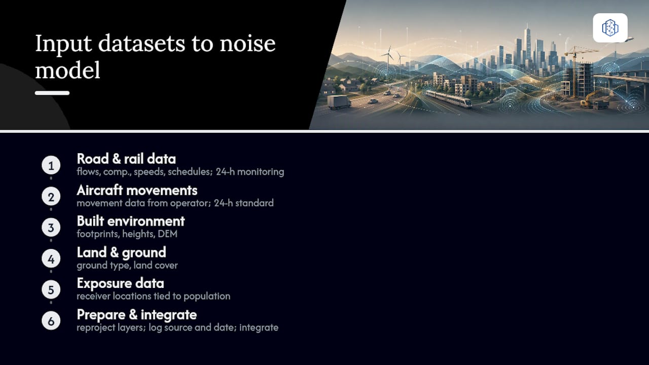
Strategic mapping guidance recommends datasets no older than three years where required.pdf), a threshold worth writing into your own project checklist even outside formal END reporting.
Measured data matters as much as modelled inputs. A full 24‑hour monitoring window is the practical standard for road, rail and aircraft sources because it captures the daytime, evening and night periods that Lden and Lnight actually weight. Shorter sampling windows are acceptable for preliminary feasibility work, but only if you scale results against a longer reference period or existing continuous monitoring nearby, and you state that scaling method in the report.
Pro Tip: Reproject every dataset into a single GIS coordinate reference system before you touch the noise model, and log the source and download date of each layer in a simple metadata table. Regulators and peer reviewers will ask for exactly this when they check your assessment.
Step 3: Choose the right calculation method and tools
CNOSSOS‑EU is mandatory for EU strategic noise mapping. It specifies separate emission and propagation models for road, rail, aircraft and industrial sources, calculated in octave or third-octave frequency bands, and it demands specific inputs on traffic composition, meteorology and ground absorption that you should have already gathered in Step 2, as set out in the CNOSSOS‑EU methodology.
Match your tool to the scope:
- Open-source libraries like NoiseModelling suit reproducible, scriptable batch runs across large areas and support dynamic updates driven by live traffic data.
- Specialist 3D noise software handles façade projections and vertical receiver grids for site-level detail.
- 3D digital-twin platforms such as 3D Cityplanner support scenario testing and stakeholder-facing visuals once the acoustic numbers exist.
Before running anything, check coordinate system consistency, receiver height conventions, and how vehicle classes in your traffic data map onto the categories your chosen method expects. A mismatch here silently corrupts results without throwing an error.
Step 4: Run the model, calibrate and report uncertainty
Calibrate your model against measured data, ideally a full 24‑hour window, and document every adjustment you make. That single discipline separates a defensible assessment from a guess dressed up in GIS layers.
The calibration procedure runs in a fixed order:
- Select monitoring sites that represent the dominant source and typical propagation conditions, not a sheltered courtyard or an anomalous junction.
- Filter recordings to strip out extraneous events (a passing siren, construction plant, a dog barking) that would bias the reference dataset.
- Run the baseline model uncalibrated and compare predicted versus measured levels at each site.
- Compute correction factors and apply them back to source emission parameters, not just as a flat offset on the output map.
Set expectations for residual error realistically. One dynamic modelling study using combined monitoring, traffic and meteorological data reported hourly mean prediction errors ranging from around −6.25 dBA to −4.46 dBA for 2D maps and a tighter 0.02 dBA to 1.93 dBA for 3D maps, in a city where over 30% of inhabitants were exposed above WHO benchmarks. Your own residuals will vary by site, but a figure in a reasonable calibration target range is typical rather than an aspiration.
Pro Tip: For aircraft noise, don’t rely on short microphone deployments alone. Request annual movement and flight-path data directly from the airport operator, since single-week measurements rarely capture seasonal runway usage patterns.
Step 5: Produce maps, exposure tables and decision-ready graphics
The outputs planners actually use fall into five categories: isodecibel contours, receiver tables listing indicator values per address or grid cell, façade vertical exposure plots, population exposure statistics, and hotspot maps flagging locations above regulatory thresholds.
Different audiences need different formats from the same underlying model run.
- Planners and designers want scenario comparison maps that show how a design choice shifts the contours.
- Regulators want exposure statistics: how many dwellings, and how many people, sit above each threshold band.
- The public needs a single, clearly legended hotspot map, not a technical frequency-band breakdown.
Deliver a mix: 2D contour maps for area overview, façade heatmaps for vertical exposure by storey, cross-section noise profiles through a street canyon, and scenario delta maps that isolate the change one mitigation option produces. Façade projections matter more than most reports acknowledge, since vertical exposure varies by storey in ways a flat ground-level contour map simply cannot show.
Step 6: Test mitigation scenarios and compare results in 3D
Use a digital twin or 3D model to run mitigation scenarios side by side and generate comparative exposure statistics before a single brick gets laid. This is where noise analysis stops being a compliance exercise and starts informing design.
Common scenario variables include:
- Changing building massing, height or orientation to self-shield courtyards and rear façades.
- Adding linear barriers along a road or rail corridor.
- Increasing green belt width between the source and receivers.
- Rerouting traffic, reducing speed limits, or changing road surface material.
- Upgrading façade glazing and ventilation on the most exposed elevations.
The practical workflow: build one calibrated baseline, change a single variable per scenario run, recalculate, then export delta maps and exposure tables that isolate exactly what each change achieved. Integrating CNOSSOS‑EU outputs with machine learning corrections and 3D visualisation has been shown to improve prediction accuracy while giving planners an immersive dashboard to compare options, which is precisely the kind of scenario testing a platform like 3D Cityplanner’s digital twin tools is built to support.
Pro Tip: Don’t assume standard attenuation figures for green infrastructure translate directly to your site. Dense planting reduces perceived and some measured noise, but the acoustic benefit is smaller and more variable than most default software assumptions suggest, so involve an acoustics specialist when a scenario relies heavily on planting for compliance.

Quality assurance, reporting and common pitfalls
A rigorous QA pass catches the errors that get reports rejected weeks after submission, not before. Run through this checklist before any model output leaves your desk:
- Check every dataset’s age against your three-year threshold and note exceptions explicitly.
- Verify coordinate systems and projections match across every layer.
- Confirm receiver heights are set correctly for façade and balcony assessments, not defaulted to ground level.
- Review calibration logs and confirm correction factors were actually applied, not just calculated.
- Version every model dataset and keep a change log for anything modified after initial calibration.
For regulatory submissions, document which version of CNOSSOS‑EU or local methodology you used, list every assumption, state the uncertainty range, and attach calibration evidence as an appendix rather than a footnote.
- Using a short, unscaled measurement window as if it were annual-average data.
- Ignoring vertical exposure and reporting only ground-level contours for a multi-storey scheme.
- Mismatching vehicle class definitions between your traffic survey and the model’s emission tables.
- Failing to record the age and source of any input dataset.
Pre-delivery checklist for reports and stakeholder meetings
Before you hand over a report or stand up in front of a planning committee, run this final pass.
- Dataset audit complete and documented, including source and date.
- Model calibrated against measurement data, with correction factors recorded.
- Exposure tables generated for every receiver category the brief requires.
- Maps carry a legend, scale bar, north arrow, stated projection and data source notes.
- Scenario delta maps produced for every mitigation option tested.
- Uncertainty statement written in plain language, not buried in an annex.
- Prepare one non-technical slide summarising what the maps mean for local residents.
- Prepare a separate technical appendix with full methodology for the regulator.
- Double-check every appendix figure matches the number quoted in the main report body.
A site analysis checklist built around these steps saves considerable back-and-forth once a scheme reaches committee stage.
Why acoustics belongs in masterplanning, not compliance
Integrate acoustic goals into masterplanning from the first massing study, not as a compliance check bolted on after layouts are fixed. Analytical noise propagation methods let planners identify noise-polluted zones early enough to shape block orientation and green belt placement before costly retrofits become the only option.
Picture a mixed-use scheme where shifting one residential block’s orientation and widening a green buffer by a few metres, tested early in a 3D model, cuts projected façade exposure on the worst-affected elevation. Visualised in a digital twin, that trade-off becomes something a planning committee can actually see, not just read in a table.
How a 3D digital twin speeds up your workflow
A browser-based digital twin removes the slowest parts of step-by-step noise analysis: pulling scattered datasets into one 3D view, testing façade exposure against real massing, and turning scenario deltas into something non-technical stakeholders instantly understand.
Three practical uses stand out. Rapid massing tests let you rotate or reposition a block and immediately see how the façade exposure shifts, without rebuilding a model from scratch. Overlaying calibrated noise contours directly onto 3D façades shows exactly which storeys and elevations exceed thresholds. Exporting comparative exposure statistics across scenarios gives planning committees and regulators a single, consistent evidence base rather than a stack of disconnected spreadsheets.
3D Cityplanner brings GIS data, 3D city models and scenario comparison into one browser-based workspace, which is exactly the environment feasibility studies and redevelopment projects need when noise mitigation has to be weighed against development capacity, greenery and parking in the same view. If you’re assembling a masterplan where acoustic performance is one variable among several, explore the digital twin city platform and start a free trial to test your own scenarios.
Sources
- NoiseModelling user guide
- Dynamic modelling for noise mapping in urban areas (ScienceDirect)
- Urban noise simulation system integrating CNOSSOS‑EU and machine learning (MDPI, 2025)
Always record the version and publication date of any standard or guidance document you rely on, since methodology updates can shift acceptance criteria between project phases.
FAQ
What Is Step-by-Step Noise Analysis?
It’s the procedural workflow planners follow to turn GIS and measured data into calibrated, decision-ready noise maps: defining scope, gathering datasets, modelling, calibrating, producing outputs and testing mitigation scenarios.
Is CNOSSOS-EU Mandatory for All Noise Assessments?
CNOSSOS‑EU is the mandatory harmonised method for EU strategic noise mapping under the Environmental Noise Directive; site-level planning assessments may use it or a more detailed local method depending on national or municipal requirements.
How Long Should Noise Monitoring Run Before Modelling?
A full 24‑hour window is the practical standard for road, rail and aircraft sources because it captures daytime, evening and night periods; shorter samples are acceptable for early feasibility work only if scaled against a longer reference dataset.
Can 3D Visualisation Actually Change Mitigation Decisions?
Yes. Testing massing, barriers and green infrastructure in a 3D digital twin like 3D Cityplanner lets planners compare exposure deltas visually before committing to a design, which speeds stakeholder buy-in compared with table-only reporting.
What’s the Difference Between a Strategic Map and a Site Assessment?
Strategic maps use annual-average Lden and Lnight indicators across a wide area for regulatory action plans; site assessments use Leq and façade-level detail tied to a specific planning application or development.